Online NLP with Linear Classifiers
All the code used in this post can be found on github here.
A good POS tagger in about 200 lines of Python demonstrates how one can use a relatively simple algorithm, the averaged perceptron, to produce a rather impressive parts-of-speech tagger. After reading it I was thinking about how one might adapt the averaged perceptron to an online setting. It was fairly easy to come up with something that seemed reasonable, but it turned out to not to work very well (at least with the data I was experimenting with). Along the way the scope significantly ballooned and I ended up doing a rather thorough survey of the current state of online discriminative linear classifiers.
Formality
In the typical online learning setting a learning algorithm is presented with a stream of examples and must output a prediction after each example. The true value is then revealed, the learner suffers an instantaneous loss, and may update its current hypothesis given this new information. This differs significantly from the traditional machine learning setting, where a learning algorithm is given access to a set of labeled examples and attempts to produce a hypothesis which generalizes well. One way to think of online learning is as a game between the learner and the (possibly adversarial) environment. Given a hypothesis class \(H\) defined on an instance space \(X\) and true (unknown) hypothesis \(\bar{h}\), at round \(t\) the game proceeds as follows:
- The environment produces an instance \(x_t \in X\)
- The learner makes a prediction based on its current hypothesis \(\hat{y}_t = h_t(x_t)\)
- The environment reveals the true output \(y_t = \bar{h}(x_t)\)
- The learner suffers loss \(l(y_t, \hat{y}_t)\)
- The learner produces a new hypothesis \(h_{t+1}\)
Given this setup the goal of the learner is to minimize the cumulative loss \(L\) over all rounds
\[ L = \sum_{t} l(y_t, \hat{y}_t) \]
In this post I’ll consider online classification where \(y\) is chosen from a finite set of mutually exclusive labels, i.e., \(y \in {1, 2, \ldots, K}\). As is common, I’ll use the 0-1 loss, \(l(y, \hat{y}) = \mathbb{I}(y \neq \hat{y})\), where \(\mathbb{I}(b)\) is the indicator function on predicate \(b\) which takes value 1 if \(b\) is true and 0 otherwise.
Data
I used two different natural language datasets for evaluation.
The first was the ubiquitous 20 Newsgroups dataset.
Specifically I used the version returned by
sklearn using the keyword arguments subset='all' and
remove=('headers', 'footers', 'quotes').
The former simply returns all the data (rather than specific subsets typically taken as training or testing), and the later strips all the metadata.
This last step makes the problem significantly more difficult and realistic
as it prevents the classifier for latching on to specific features that are idiosyncratic to the particular data set (like specific email addresses) and not generally interesting for identifying topics.
The second was a collections of reviews taken from Amazon available
here.
The goal is to predict whether each review is positive or negative.
I grabbed everything between the <text_review> and </text_review> tags and ignored the unlabeled documents.
For preprocessing I used sklearn’s
CountVectorizer class.
The code looks like
from sklearn.feature_extraction.text import CountVectorizer
vectorizer = CountVectorizer(token_pattern=r'(?u)\b\w+\b')
preprocess = vectorizer.build_preprocessor()
tokenize = vectorizer.build_tokenizer()
getwords = lambda doc: ' '.join(tokenize(preprocess(doc)))
Given a document getwords returns a string of space delimited lowercase words.
As a final preprocessing step I’ve ignored word frequency information, resulting in a binary bag-of-words feature vector.
Here’s a summary of the data:
| Dataset | Labels | Documents | Vocab Size |
|---|---|---|---|
| 20news | 20 | 18846 | 134449 |
| Reviews | 2 | 8000 | 39163 |
Learners
I’ll benchmark a few different classifiers that are suited to the online setting. They’re all linear classifiers, so in essence the algorithms can be thought of as different ways for searching in the same hypothesis class. A nice property of linear algorithms is the parameter updates normally only depend on the number of non-zero elements of the feature vector. This is a serious win when working with sparse data like one typically encounters when doing NLP. It means even if the feature vectors are really large we only need to update \(O(S)\) parameters, where \(S\) is the number of non-zero features (I’ll use \(S\) for this purpose throughout). This makes linear algorithms a natural choice in the online setting, where updates happen after seeing each example.
Perceptron
The perceptron is the canonical online linear classifier. The perceptron has the nice property that the number of parameters that get updated after processing each example doesn’t depend on the number of classes. When it makes a mistake it updates \(2S\) parameters. When no mistake is made, it doesn’t have to do anything. This means the perceptron will be the most efficient algorithm on the list in terms of work per round. There are also no hyperparameters to tune.
Multiclass Logistic Regression
Using stochastic gradient descent to fit a logistic regression model is typically my go-to technique for online classification problems. Unfortunately if there are \(K\) classes, then after each example the algorithm updates $KS$ parameters. Furthermore these updates happen regardless if the model gets the prediction correct or not. This can be a serious cost, especially if \(K\) is very large (like in language modeling tasks for example).
Passive-Aggressive Algorithms
Passive-Aggressive algorithms are a more recent (2003) family of margin based linear classifiers geared toward the online setting. Whenever the margin constraint is violated the PA algorithm updates \(2S\) parameters, otherwise it doesn’t do anything. This means the complexity will be comparable to that of the perceptron, with the added caveat it may do some work even when a prediction is correct due to the margin constraint. I used the third variant described in the paper (PA-II).
Confidence Weighted
Confidence weighted algorithms are another more recent linear classifier. Like passive-aggressive algorithms they are margin based, but are augmented by maintaining a distribution over the parameters. The claim that this produces better classifiers in an NLP setting largely seems to agree with my experiments. In particular I used the multi-class version presented here with the single-constraint update and a diagonal approximation to the full covariance matrix. The parameter updates have the same complexity as the passive-aggressive algorithm with the additional overhead of needing to update both the means and covariance. I ran into a few hangups when implementing the algorithm, which is still quite rough currently (not that any of it is polished).
Online Averaged Perceptron
The averaged perceptron works by storing the parameters from every round. To make predictions it uses the average of all these parameters vectors
\[ \hat{y} = \arg\max_k \left\lbrace\frac{1}{T}\sum_{t=1}^T \theta_t \cdot \phi(x, k)\right\rbrace. \]
A natural way to generalize the averaged perceptron to the online setting is to store two sets of parameters. One is a set of normal perceptron parameters. The other is the sum of the first set of parameters across all rounds. When presented with an example we make two predictions. The first uses the normal perceptron parameters, which will only be used for updates. The second uses the averaged parameters and is taken as the actual prediction. When given the true label we update the normal parameters with a traditional perceptron update as if we used the first prediction, and the add these new parameters values to the totals. By being smart and using timestamps to track the last time a specific parameter was updated when storing the totals, this scheme does twice as much work as a normal perceptron.
Results
The perceptron and averaged perceptron don’t have any hyperparameters, so there was nothing to tune there.
For logistic regression I needed to tune the learning rate \(\eta\),
for the passive-aggressive algorithm I needed to tune the aggressiveness parameter \(C\), and for the confidence weighted classifier I needed to to tune the confidence parameter \(\eta\).
In all cases I used the same small subset of the data and did some random search based on intuition and recommendations from the literature. Interestingly, I found the same parameters to work well on both datasets for the passive-aggressive algorithm and confidence weighted.
For logistic regression I needed to reduce the learning rate to get decent performance on the review dataset.
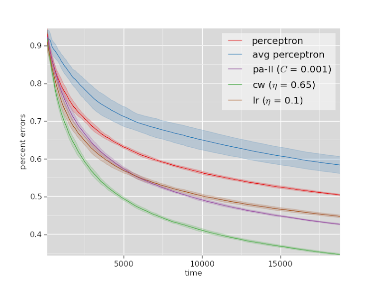
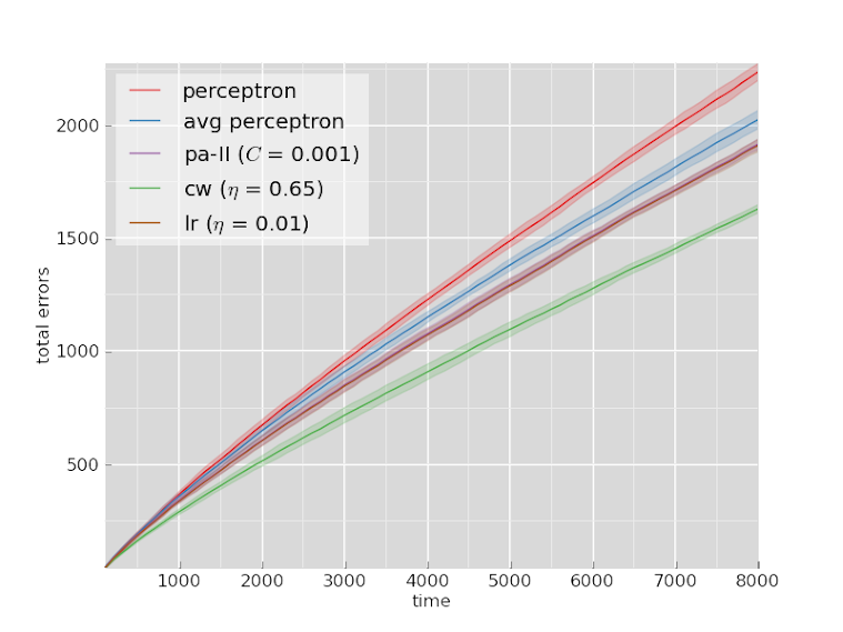
To assess each model I simply made a single pass over the full dataset and recorded the total number of errors at time \(t\). I repeated this 10 times for different permutations of the data and plotted the mean and standard deviation. Plots below include both totals errors as well as the percentage of errors (total errors divided by number of rounds).
20Newsgroups

Reviews

Conclusion
The rankings are mostly the same across both datasets.
The confidence weighted classifier outperforms all the other algorithms by a clear margin on both datasets.
Logistic regression and the passive-aggressive algorithm perform comparably, and the averaged perceptron and the normal perceptron are both worse than everything else.
The poor performance of the averaged perceptron in an online setting isn’t necessarily surprising, but I still wonder if something could be done to fix it. Perhaps using something like an
exponential moving average
to give higher weight to more recent parameter settings, which have seen significantly more data.
One thing worth noting is that it may have helped adding a regularization term to the logistic regression model. I didn’t do this for two reasons. First, I wanted to keep the number of hyperparameters low. As it is each algorithm has at most one hyperparameter. Second, I’ve frequently found that regularization isn’t as helpful when using SGD, especially in an online setting.